
Finetuning with LoRA and variants
The article "Finetuning with LoRA and Variants" discusses Low-Rank Adaptation (LoRA), a technique that efficiently fine-tunes large language models by adding a small number of trainable parameters, reducing computational costs. It also explores LoRA+ and other innovations enhancing model adaptation.

Imagine you've spent countless hours training a large language model, pouring in vast amounts of data and computing power, only to realize that you must fine-tune it for a specific task. Traditional fine-tuning methods often require updating all the model parameters, which can be time-consuming and resource-intensive, especially for large models. This is where Low-Rank Adaptation (LoRA) comes in as a game-changer. LoRA is an innovative technique that efficiently adapts pre-trained language models to new tasks by adding a small number of trainable parameters, reducing the fine-tuning process to a fraction of its original computational cost.
In this blog post, we'll explore (or, as ChatGPT calls it, "delve into" ) LoRA's workings and its variants for fine-tuning large language models.

🔅 Low-Rank Adaptation (LoRA)
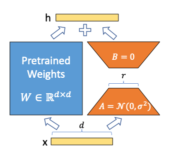
LoRA emerged as a technique to adapt pre-trained models to specific tasks without the computational overhead of retraining millions to billions of parameters. By introducing smaller, tunable matrices \((A, B)\) alongside the pre-trained weight matrix \(W\), LoRA allows for efficient model adaptation with a reduced number of parameters. It hypothesizes that the fine-tuning process primarily involves low-rank updates and captures these through the matrices A and B, where \( A \in \mathbb{R}^{m \times r} \) and \( B \in \mathbb{R}^{r \times n} \), with \( r \) being significantly smaller than both \( m \) and \( n \). This approach minimizes the initial impact on the model's output as \( AB \) starts as a zero matrix due to the initialization of B with zeros.
The forward pass in a model fine-tuned with LoRA is modified as \( h = (W + AB)x \), incorporating the low-rank updates directly into the computation. This is computationally less intensive because it reduces the number of trainable parameters, sometimes by orders of magnitude, and lessens GPU memory usage. Despite the fewer parameters, LoRA can achieve performance on par with or better than full-parameter fine-tuning. This is because only a small subset of the parameters—those most relevant to the new task—are updated, while the bulk of the parameters, which capture general knowledge, remain unchanged.
Linear adapter fine-tuning, a method under which LoRA falls, adds adaptability to the model by incorporating trainable parameters into key layers like self-attention and feed-forward networks. These adapters can be linearly combined with the existing weights of the model, allowing for a reparametrization back into the original model structure post-fine-tuning. Thus, LoRA preserves the architecture of the base model while providing a path for efficient adaptation, demonstrating its effectiveness as a parameter-efficient fine-tuning method that leverages the intrinsic low-rank structure of the weight updates.
To use it using Huggingface's Autotrain, use the below bash template:
autotrain llm \
--train \
--model ${MODEL_NAME} \
--project-name ${PROJECT_NAME} \
--data-path data/ \
--text-column text \
--lr ${LEARNING_RATE} \
--batch-size ${BATCH_SIZE} \
--epochs ${NUM_EPOCHS} \
--block-size ${BLOCK_SIZE} \
--warmup-ratio ${WARMUP_RATIO} \
--lora-r ${LORA_R} \
--lora-alpha ${LORA_ALPHA} \
--lora-dropout ${LORA_DROPOUT} \
--weight-decay ${WEIGHT_DECAY} \
--gradient-accumulation ${GRADIENT_ACCUMULATION} \
--quantization ${QUANTIZATION} \
--mixed-precision ${MIXED_PRECISION} \
$( [[ "$PEFT" == "True" ]] && echo "--peft" ) \
$( [[ "$PUSH_TO_HUB" == "True" ]] && echo "--push-to-hub --token ${HF_TOKEN} --repo-id ${REPO_ID}" )
⚡️ Innovations Beyond LoRA
LoRA+
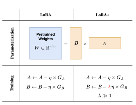
LoRA+ introduces differentiated learning rates for matrices A and B, improving training efficiency and model accuracy by adjusting the learning rate of matrix B significantly higher than that of matrix A. Empirically, \( \lambda = 16\) is found to be the best choice.
Readers can refer to LLAMA-Factory scripts to use LoRA+.
#!/bin/bash

CUDA_VISIBLE_DEVICES=0 python ../../src/train_bash.py \
    --stage sft \
    --do_train \
    --model_name_or_path meta-llama/Llama-2-7b-hf \
    --dataset alpaca_gpt4_en,glaive_toolcall \
    --dataset_dir ../../data \
    --template default \
    --finetuning_type lora \
    --lora_target q_proj,v_proj \
    --output_dir ../../saves/LLaMA2-7B/loraplus/sft \
    --overwrite_cache \
    --overwrite_output_dir \
    --cutoff_len 1024 \
    --preprocessing_num_workers 16 \
    --per_device_train_batch_size 1 \
    --per_device_eval_batch_size 1 \
    --gradient_accumulation_steps 8 \
    --lr_scheduler_type cosine \
    --logging_steps 10 \
    --warmup_steps 20 \
    --save_steps 100 \
    --eval_steps 100 \
    --evaluation_strategy steps \
    --load_best_model_at_end \
    --learning_rate 5e-5 \
    --num_train_epochs 3.0 \
    --max_samples 3000 \
    --val_size 0.1 \
    --plot_loss \
    --fp16 \
    --loraplus_lr_ratio 16.0
Note the loraplus_lr_ratio as non-zero to active LoRA+
This is how the custom optimizer is created:
def _create_loraplus_optimizer(
    model: "PreTrainedModel",
    training_args: "Seq2SeqTrainingArguments",
    finetuning_args: "FinetuningArguments",
) -> "torch.optim.Optimizer":
    if finetuning_args.finetuning_type != "lora":
        raise ValueError("You should use LoRA tuning to activate LoRA+.")

    loraplus_lr = training_args.learning_rate * finetuning_args.loraplus_lr_ratio
    decay_args = {"weight_decay": training_args.weight_decay}

    decay_param_names = _get_decay_parameter_names(model)
    param_dict: Dict[str, List["torch.nn.Parameter"]] = {
        "lora_a": [],
        "lora_b": [],
        "lora_b_nodecay": [],
        "embedding": [],
    }
    for name, param in model.named_parameters():
        if param.requires_grad:
            if "lora_embedding_B" in name:
                param_dict["embedding"].append(param)
            elif "lora_B" in name or param.ndim == 1:
                if name in decay_param_names:
                    param_dict["lora_b"].append(param)
                else:
                    param_dict["lora_b_nodecay"].append(param)
            else:
                param_dict["lora_a"].append(param)

    optim_class, optim_kwargs = Trainer.get_optimizer_cls_and_kwargs(training_args)
    param_groups = [
        dict(params=param_dict["lora_a"], **decay_args),
        dict(params=param_dict["lora_b"], lr=loraplus_lr, **decay_args),
        dict(params=param_dict["lora_b_nodecay"], lr=loraplus_lr),
        dict(params=param_dict["embedding"], lr=finetuning_args.loraplus_lr_embedding, **decay_args),
    ]
    optimizer = optim_class(param_groups, **optim_kwargs)
    logger.info("Using LoRA+ optimizer with loraplus lr ratio {:.2f}.".format(finetuning_args.loraplus_lr_ratio))
    return optimizer
DoRA
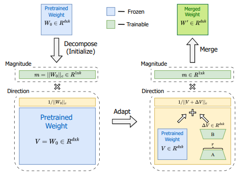
DoRA decomposes weight updates into magnitude and direction, allowing for independent tuning and closer alignment with fine-tuning practices.
NEFTune
NEFTune, or Noisy Embedding Instruction Finetuning, is an algorithm designed to fine-tune pre-trained models using a technique that introduces noise into the embedding space of the model. The process begins by initializing the model parameters from a pre-trained model. During each iteration, a minibatch of data is sampled from the dataset \( D \), consisting of tokenized input-output pairs \( (X_i, Y_i) \). The algorithm then retrieves the embeddings \( X_{\text{emb}} \) for the input batch, which is a tensor with dimensions corresponding to the batch size \( B \), sequence length \( L\), and embedding dimension \( d \).
A key step in NEFTune is the injection of noise into the embeddings. It generates a noise vector \( \varepsilon \) with uniform distribution between -1 and 1, scaled by the hyperparameter \( \alpha \), and adjusted by the square root of the product of sequence length \( L \) and embedding dimension \( d \). This noise is then added to the original embeddings, producing a noised version \( X'_{\text{emb}} \).
With the noised embeddings, the model \( f_{/\text{emb}}( \cdot ) \) makes predictions \( \hat{Y}_i \), and the parameters \( \theta \) are updated using an optimizer function based on the loss between the predictions and the ground truth labels \( Y_i \). This process iterates until a stopping criterion is met or a maximum number of iterations is reached. It's important to note that if a batch contains sequences of varying lengths, the noise scale is computed independently for each sequence to accommodate the difference in sequence lengths.
NEFTune leverages the noise-injection strategy to potentially enhance model robustness and generalization. This strategy pushes the model to learn from a slightly perturbed embedding space and thus potentially improve its ability to make predictions on unseen data.
To enable it in Trainer, set the neftune_noise_alpha parameter in TrainingArguments in Huggingface to control how much noise is added.
from transformers import TrainingArguments, Trainer

training_args = TrainingArguments(..., neftune_noise_alpha=0.1)
trainer = Trainer(..., args=training_args)
PiSSA
PiSSA (Principal Singular values and Singular vectors Adaptation) introduces a parameter-efficient fine-tuning (PEFT) method for LLMs, aiming to optimize a significantly reduced parameter space while maintaining or surpassing the performance of full-parameter fine-tuning. This approach is grounded in the idea that pre-trained, over-parametrized models inhabit a low intrinsic dimensional space. PiSSA operates by decomposing a pre-trained matrix \(W \in \mathbb{R}^{m \times n}\) into two trainable matrices \(A \in \mathbb{R}^{m \times r}\) and \(B \in \mathbb{R}^{r \times n}\), where \(r \ll \min(m, n)\), in addition to a residual matrix \(W_{\text{res}} \in \mathbb{R}^{m \times n}\) for error correction. Singular value decomposition (SVD) is used to factorize \(W\), with its principal singular values and vectors initializing (A) and (B), and the residual singular values and vectors initializing \(W_{\text{res}}\), which remains unchanged during fine-tuning.
Contrastingly, LoRA (Low-Rank Adaptation), another PEFT method, hypothesizes that changes in model parameters (\(\Delta W\)) form a low-rank matrix and approximates \(\Delta W\) through the product of two matrices (A) and (B), initialized with Gaussian noise and zeros, respectively. However, PiSSA differentiates itself by initializing (A) and (B) with the principal singular values and vectors of the original matrix (W), allowing for a better approximation of the outcomes of full-parameter fine-tuning by modifying the essential parts of the model while keeping the "noisy" parts unchanged. This strategic approach enables PiSSA to achieve faster convergence and superior performance compared to LoRA, as demonstrated by its effectiveness on various benchmarks, where it outperformed LoRA across all tests with the same setups but different initializations.
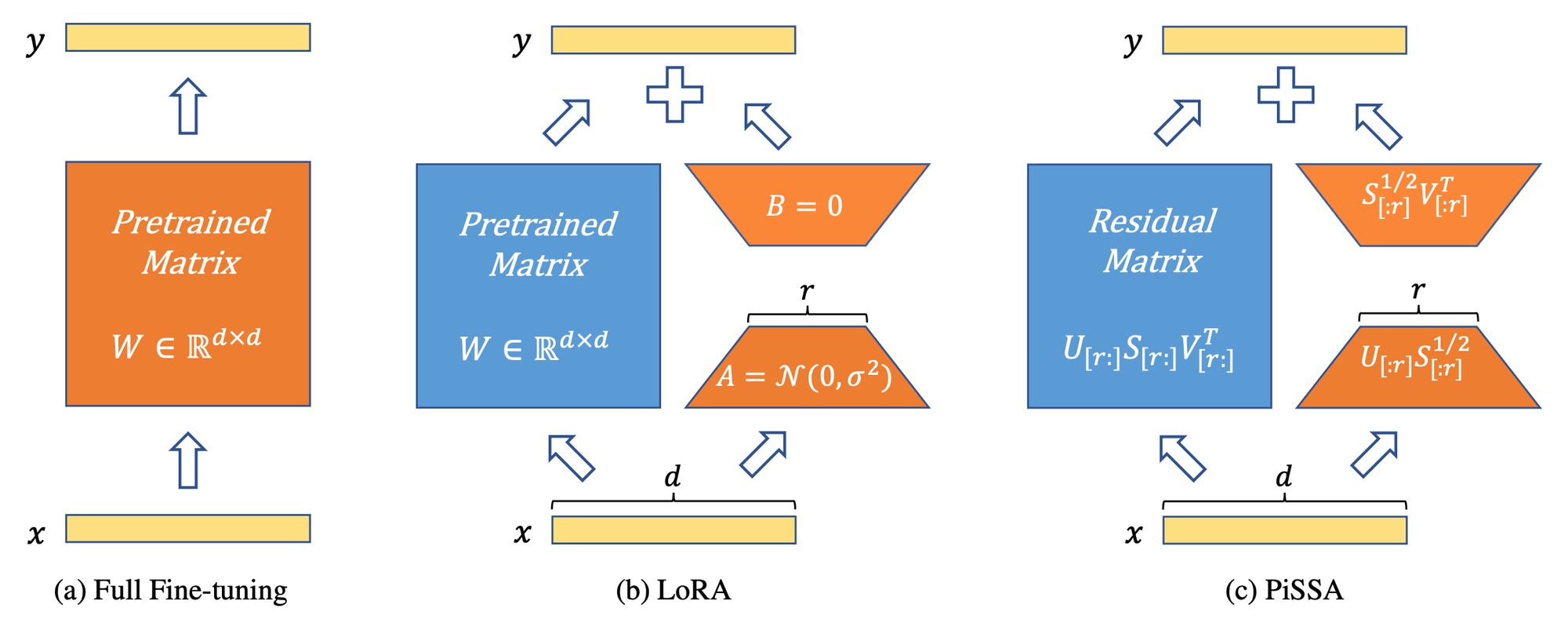
Figure 5 below presents a comparative performance analysis of GSM8K accuracy among three different models: LLaMA 2-7B, Mistral-7B-v0.1, and Gemma-7B, each fine-tuned using different methods—Full Fine-tuning, LoRA, and PiSSA—across various ranks. The dashed green line represents the accuracy achieved through full fine-tuning, serving as a benchmark. The blue bars indicate the accuracy attained by LoRA, and the orange bars represent the accuracy obtained with PiSSA. As the rank increases, so does the model's capacity to capture more information, reflected in the general trend of increasing accuracy.
PiSSA's superior performance is consistent across all three models and at varying ranks, showcasing that even at lower ranks, PiSSA achieves or exceeds the accuracy of full fine-tuning, surpassing LoRA's performance. Notably, in the Mistral-7B-v0.1 model, PiSSA achieves a sharp increase in accuracy as the rank grows, aligning closely with the full fine-tuning performance and even outperforming it at higher ranks. This trend indicates PiSSA's efficient parameter adaptation, capitalizing on the most significant components of the pre-trained model's matrix to improve learning speed and final model performance.
To learn more about static datasets similar to GSM8K used to evaluate LLMs, refer to our blog on LLM Evaluations (linked below).
 Sayantan Das
To utilize PiSSA with peft, the authors give out some instructions:
- Clone this custom fork of huggingface's peft library.
pip install git+https://github.com/fxmeng/peft.git- Initializing PiSSA and the residual model with SVD:
# Download the standard llama-2-7b model from huggingface:

import torch
from transformers import AutoTokenizer, AutoModelForCausalLM
model = AutoModelForCausalLM.from_pretrained('meta-llama/Llama-2-7b', device_map="auto")
tokenizer = AutoTokenizer.from_pretrained('meta-llama/Llama-2-7b')
tokenizer.pad_token_id = tokenizer.eos_token_id

# Inject PiSSA to the base model:

from peft import LoraConfig, get_peft_model
peft_config = LoraConfig(
    r = 16,
    lora_alpha = 16, # lora_alpha should match r to maintain scaling = 1
    lora_dropout = 0,
    init_lora_weights='pissa', # PiSSA initialization
    task_type="CAUSAL_LM",
)
model = get_peft_model(model, peft_config)
model.print_trainable_parameters()- Finetune PiSSA on Alpaca Dataset:
from trl import SFTTrainer
from datasets import load_dataset
dataset = load_dataset("fxmeng/alpaca_in_mixtral_format", split="train")
trainer = SFTTrainer(
    model=model,
    train_dataset=dataset,
    dataset_text_field="text",
    max_seq_length=1024,
    tokenizer=tokenizer
)
trainer.train()
🔮 Conclusion
Several questions remain to be verified in the future: 1) Can variants of LoRA significantly improve a broader range of tasks and larger models? 2) When the iteration steps of LoRA are sufficiently long (adequately fitting the data), can they match the performance of more advanced versions? 3) Can combining different successors of LoRA lead to further enhancement? 4) How to explain theoretically the advantages of these advanced versions over the original LoRA? We are actively exploring these questions. Nevertheless, we are excited to see the huge potential of the advanced LoRA variants already demonstrated in existing experiments, and look forward to more tests and suggestions from the community.