
Mamba Simplified - Part 1 - Essential Pre-Requisites
This article introduces foundational concepts like derivatives, differential equations, and neural networks, essential for understanding Mamba—a Small Language Model based on State Space Models (SSMs). It serves as a refresher to grasp Mamba's architecture effectively.

The previous blog post describes how Small Language Models (a.k.a SLMs) hold potential in the generative AI space. We discussed the emergence of the idea of SLMs and how synthetic data can be a driving factor in producing powerful small language models (for example: Phi-2 by Microsoft). Just a month ago, another new Small Language Model entered the Gen-AI space called Mamba. Now, the interesting part is that the model is not based on transformers using the Attention mechanism. Instead, this is based on State Space Models (SSMs).
Personally, when I started to read the paper, it was an outburst of different cross-domain concepts with a bunch of mathematical equations. We divided the blog post into two parts to keep it short and easy to understand. The first part will include all the required prerequisites to understand how Structured State Space Models (S4) work. It will also be a great refresher for some popular topics of differential equations and traditional concepts of RNNs and CNNs. Let's dive in.
📈 Derivatives
Derivatives simply measure the rate at which a function changes w.r.t. its input variables. Consider this animation below.
As you can see in the above figure, we have a function f(x) and we are finding the derivative of it at all points of x. To put it more simply, the dotted (red/green) line you see in the above gif denotes the slope of the graph along that point. This slope (the dotted line) represents the direction and the steepness of the graph or function at that point.
Two ways of computing derivative
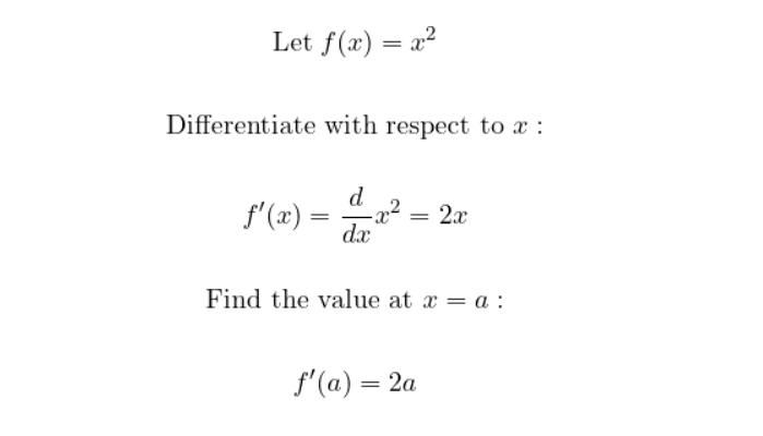
Let's assume a simple function f(x) = x^2. Now there are two ways of calculating its derivative, viz: The analytical way and the numerical way. Figure 2, below shows both the computation.
Analytical Method
Let's solve the problem using the analytical method first.
Numerical Method
Here is the numerical method of solving the same problem.
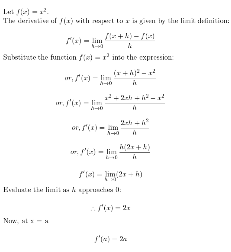
Now, analytical methods are theoretically precise and easier to calculate (although not always). However, computationally we can not have a d/dx operator. So we use an analytical method that tries to approximate the same value of the derivative of a function at some point (here 'a') using a very small value of h (which tends -> to zero). We can also say that the second method (a.k.a the numerical method) is the "discretized" form of the continuous analytical method.
Please keep an eye on the word "discretization" and the numerical method shown above. Those two are super important for later understanding of some parts of Mamba.

⏳Differential equations

Now that we have understood what derivatives are, let's understand differential equations. Real-world natural systems (e.g. population growth or flow of some fluid) and artificial systems (e.g. Flow of traffic or transfer of heat of a certain mechanical system, etc) require predictability for obvious tracking reasons. These systems are heavily changing their states. For this reason, we can not just model these systems with some random equations.
Consider the fact that these systems are not static; they change continuously over time. This is where the concept of rates of change, which we explored with derivatives, comes into play. Differential equations essentially express how a quantity changes concerning another variable, often time. So the input of differential equations are the basic inputs like x, y, etc, along with the derivates. Here is a scenario to understand this better.
The scenario
Imagine you are in a laboratory and you are responsible for modeling the population of rats. The population (or the rate of change of the rats) grows at a constant rate lambda proportional to the number of bunnies. Let's consider the following variables:
- The number of rats at
t = 100, is 5 lambda = 2
In the above problem, we can say that the rate of change of the number of rats w.r.t time is proportional to the number of rats itself. So we can then say:
The number of new rats born at a particular time (t) is lambda times the number of rats on the same time step (t). Mathematically we can write,

Now, as you can see above, we modeled a differential equation. The solution of the differential equation will be a function that will model the population growth of the rats. Solving this equation can also be done in two methods. And, you guessed it right. Analytical and Numerical method.
Analytical Method

Numerical method
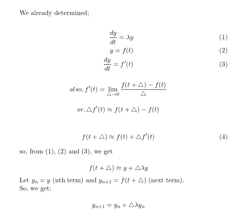
Now knowingly or unknowingly you just derived Euler's method (for the given function). And this is what the general Euler's equation looks like
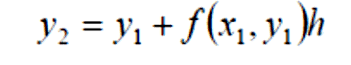
Very similar to the one we derived here, just instead of h, in our case, it is the variable delta. So congratulations if you made till here. Now we have derived it, how to find the solution to it? Well, it is tough on pen and paper. Finding the solution is an iterative method, where we start from 0 (where our initial solution is given), all the way to t = 100 where the step size is delta. So, the solution depends on the variable delta. The lesser the value of delta is, the more precise the value will be. We are smart people, let's write a Python function to get the answer.
def compute_the_number_of_new_rats(x0, t, delta, lambda_ = 5):
    """A numerical function to compute the number of rats at time t.

    Args:
        x0: The initial number of rats at t = 0
        t: The total number of time t
        lambda_: The value of proportionality constant lambda (Default set to 5)
        delta (_type_): The step size.

    Returns:
        Float: Approximate number of rats at time t.
    """
    total_number_of_steps = int(t/delta)
    for _ in range(total_number_of_steps + 1):
        xt = x0 + delta * lambda_ * x0
        x0 = xt
    return xt

if __name__ == '__main__':
    delta = 0.0005
    t = 100
    x0 = 5

    y_t100 = compute_the_number_of_new_rats(x0, t, delta)

    print(f"After t = {t}, total number of new rats took birth are: {y_t100}")
Now, suppose the value of the delta is 0.0005 and if you run this code by putting all the inputs you will see that the results are approximately coming as 3.769 which is an approximation to the analytical method.
Since numerical computation is by definition calculating the approximation of analytical methods, there are several other numerical methods other than Euler's method. Some of the popular and better alternatives to Euler methods are the Runge-Kutta Method, Adams-Bashforth Method, etc. Essentially, we are "discretizing" a continuous function and the above methods can be thought of as different discretizing rules.
⛓ A brush-up on Recurrent neural networks
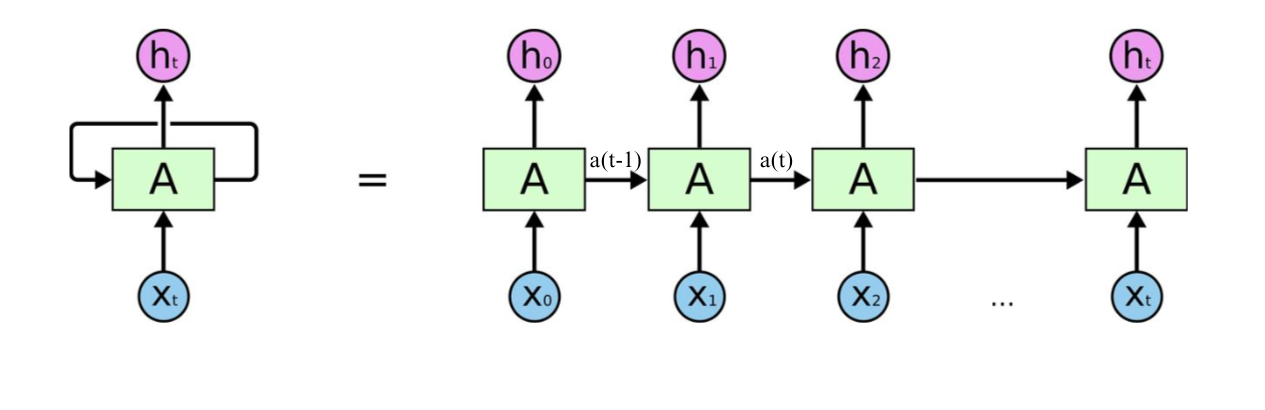
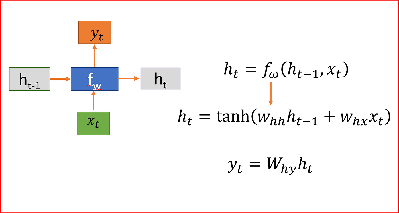
Recurrent Neural Networks were super popular earlier in the time before Attention came into the scenario. Simply put, an elementary block of a recurrent neural network (RNN) is based on a "recurrent" operation. The inputs for block A at time t are the current input xt and the previous hidden state at-1 .
Long Context Length was the biggest problem in the case of RNNs or any recurrent networks (like GRUs or LSTMs). The reason behind this is vanishing gradient descent. Another notable limitation of RNNs is the extended training time, which results from the inability to parallelize recurrent operations. In feed-forward propagation, the computation of each state is contingent upon the completion of the previous step, a requirement that also applies to backpropagation. Therefore, the training complexity of RNNs is O(N).
Transformers stood out for the above two reasons. Relative to RNNs or LSTMs, Transformers are better with longer context lengths and are parallelizable during training. However, it's worth noting that in one aspect, RNNs/LSTMs still hold an advantage over Transformers: inference time. RNNs maintain a constant inference timeO(1), due to their dependence only on the previous state during inference. On the other hand, Transformers exhibit O(N) complexity during inference time. In the Transformer architecture, each newly generated token cumulatively serves as the input for the subsequent token generation. Hence, the complexity is proportional to the context length of the provided prompt.
💡A brush up on Convolutional networks
Convolutional Neural Networks (CNNs) have been essential in the field of Deep Learning since its early days. Think back to AlexNet – it was one of the first networks that excelled in the ImageNet challenge, surpassing other techniques. If you work in machine learning or deep learning, you've probably come across the term 'convolution' mainly about Convolutional Neural Networks.
The learnable 2D convolution kernels, which slide over the image (as shown in the animation above), simplify the input image into several key features. In tasks like distinguishing between cats and dogs, these features include ears, noses, and eye shapes - elements that set these animals apart. With adequate training, these kernels can capture these distinguishing characteristics, making classification by the model more straightforward. Additionally, a significant advantage of convolutions is that the training of a Convolutional Neural Network can be parallelized easily.
1D Convolution
Tracing back to the basics, it's clear that all types of CNNs (1D, 2D, or 3D) originate from the fundamental convolution operation. This operation acts like a mathematical filter, scanning and merging information from one set of data to another. Simply put, in convolution, a small filter (known as a kernel) slides across the data, multiplying and adding values to emphasize specific features. The particular features highlighted, and their significance, depend on the characteristics of the filter or kernel.
If you want to get a better intuition on how the convolution operator works and how it is used in some real-world scenarios (step-by-step), you can check out this awesome article by BetterExplained.
💾 A primer on GPU Memory hierarchy and Kernel fusion technique
If you are into deep learning then you might have heard about terms like "writing custom kernels" or "kernel fusion". If not, do not worry, we got you. Have you ever wondered why there is so much craze when Nvidia releases a new GPU? Does it make things faster? Yes. But what's that important thing (out of a lot of other aspects) that makes an A100 better than a RTX-3080?
It is the bandwidth. Modern GPUs are super fast doing matrix/tensor operations. We quantify that with the number of floating point operations per second or FLOPs. Now, what is bandwidth? This is essentially the cost of moving the data (tensors or matrices) from one place to another. Consider this figure below.
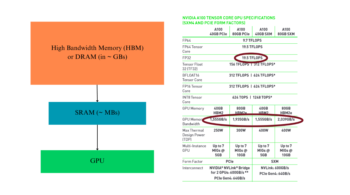
In the above figure you can see that in all the variants of A100 GPUs, one constant thing is the FLOPs. However, the memory bandwidth makes the differentiating factor (and so becomes the prices). In the above figure, you can see a very simplified hierarchy of the GPU memory. Before doing any operations, all the tensors or matrices (or whatever is required before doing the actual computation) are first stored and transferred from the DRAM to SRAM.
The DRAM or the High Bandwidth Memory is what shows up in our nvidia-smi. Now the movement of data from DRAM to SRAM is relatively slow which is responsible for the overhead. Once loaded, SRAM (whose memory is in MBs) loads that to GPU for actual computations and then from GPU to SRAM to HBM. In all of the processes, what causes the overhead is loading data to and from HBM (memory bandwidth cost). Unfortunately, a lot of times, the algorithms (e.g., computing attention) that we use in deep learning may not cause problems in the number of operations we do, but instead how many tensors we move around in the different memory hierarchy. We say those operations i/o bound operations.
Suppose your neural network does three sequential operations, then here are the steps that happen in a naive approach. See the figure below.
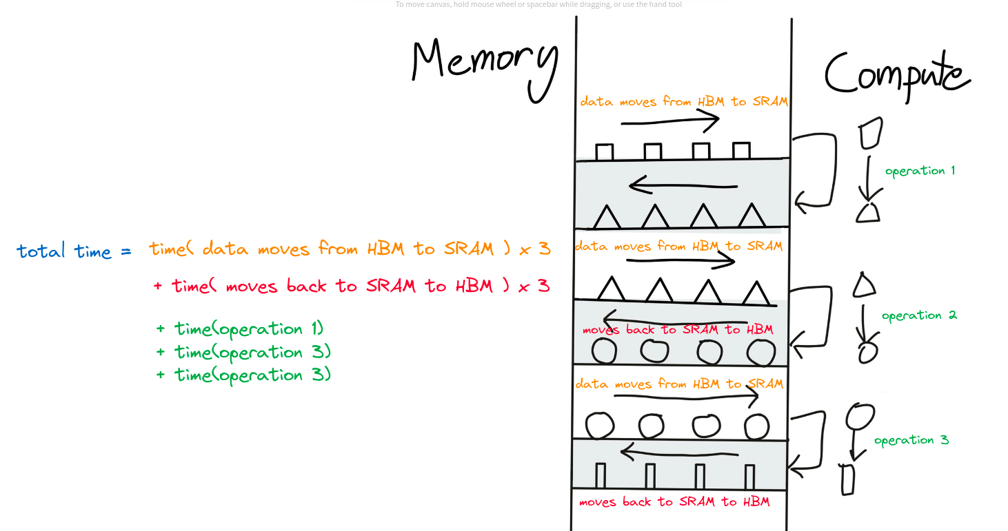
To do 3 sequential operations, we need to move data from a total of 6 times (3 times from HBM to SRAM and 3 times from SRAM back to HBM). This approach is not optimized. And we can easily see that there is an unwanted redundancy happening here. Instead what we can do is simply do all three operations one by one and load back to SRAM all at once (since we do not care for the intermediate outputs). Which something looks like this:
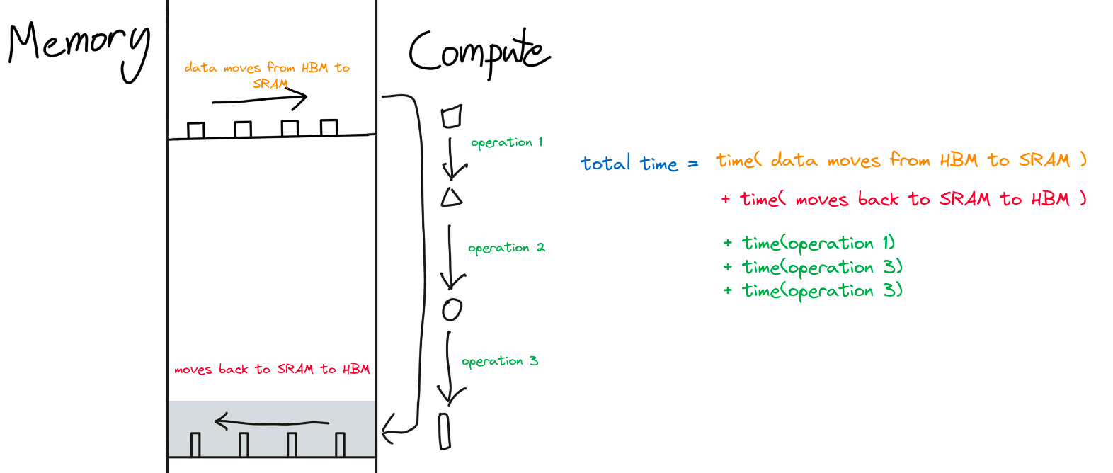
This is very obvious that the total time to operate in the naive way will be way more than the latter. Since actual FLOPs are tremendously fast compared to the copying speed. This optimization is called "Kernel Fusion".
Most operations already come with Kernel fused (wherever required). However, sometimes, when we come up with new research, those are heavily required. And sometimes, we also come up with better optimization compared to present operations. For example FlashAttention and FlashAttention v2. You can check out the linked paper, but we would not explain this here, since it is out of the scope of the topic.
🔮 Conclusion
This post was dedicated to having a quick revision to the mathematical tools required for understanding the Mamba architecture. Although all of these topics are subjects of their own. But, we feel that this introduction should be more than enough to understand Mamba easily. If you want to go into more depth, you can check out our references section which contains some good resources we took inspiration from. In the next post, we will cover the State Space Models (precursors of the Mamba), followed by how the Mamba was made as a modification of the S4 model. Until that, Stay Tuned.