Mamba Simplified - Part 2 - S4 and Mamba

Mamba is a very recent deep-learning architecture and it is fundamentally different from transformer-based models. Mamba's performance is on par with the current Small/Large Language models like Phi-2, Mistral, Llama 2, etc. The Structured State Space for Sequence Models (S4), a State Space Model, is considered the precursor of Mamba.

In this blog, we will understand what State Space Models are, and dive into the S4 and the Mamba architecture. Please note that both papers (S4 and Mamba) use a lot of concepts from differential equations, convolutions, recurrence, and GPU-based optimization operations like Kernel Fusion. If you want a quick refresher on these concepts to understand this blog properly, check out our previous blog, which covers all of those.

🎷 Sequence and Signals

Let’s start by understanding the goal of a sequence model. Fundamentally, a sequence model tries to map an input (discrete/continuous) signal to another (discrete/continuous) signal. An example of discrete signals is a set of tokens obtained from a prompt. Whereas we can think of musical notes as a continuous signal. However, in the end, those continuous signals are converted to discrete counterparts (through sampling), because computers cannot take continuous phenomena as input. One example of sequence modeling is language completion where given some sequence of tokens, we need to output some other sequence of tokens, that “makes sense”. Other similar examples could be: Music Generation, and /or DNA Modeling.

🚀 State Space Models

From Wikipedia definition, we define State Space Models (SSMs) as:

A mathematical model of a physical system specified as a set of input-output, and variables related by first-order differential equations.

Or simply, State Space models help us to model physical systems with a defined set of input and output and those are related by a first-order differential equation. Since differential equation tells us a system's behavioral change w.r.t. time (example population modeling). Mathematically we define a State Space Model with the given equations.

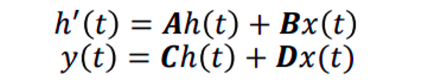
The figure above shows a first-order differential equation. The variables A, B, C, and D are known as State variables. They are responsible for memorizing the state of the system and modeling it accordingly. Hence, they are kept as learnable parameters during model training.

Figure 1 is a first-order differential equation. To find the output signal y(t), we need first solve and find out x(t). The variable u(t) is our input state. However, solving this differential equation is hard analytically (unlike our example in the previous blog). The figure below solves this equation numerically.

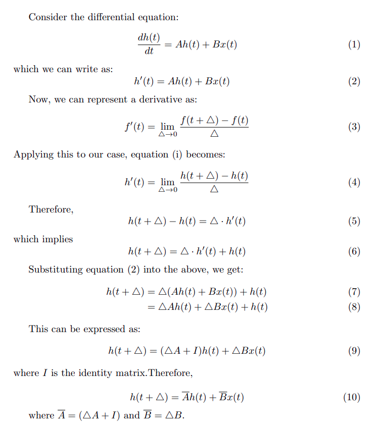
Congratulations. Knowingly or unknowingly, you have derived the solutions of the State Space Models. Here is what the actual solution looks like:

Where ht-1 can be viewed as a hidden state and A_bar is the transition matrix. In Figure 2, you saw how we defined A_bar. But in the actual S4 paper, it is represented using the bilinear method (instead of our Euler method). On the other hand, Mamba uses a different method called Zero-Order Hold. However, this method of converting the variables A, B, and to these discrete A_bar, B_bar, and C_bar is called discretization.

Subscribe to Prem Newsletter

Subscribe

Email sent! Check your inbox to complete your signup.

No spam. Unsubscribe anytime.

🔮 An Ideal Language Model

Transformers became popular due to the highly parallelizable architecture during training, and because they don't suffer from vanishing/exploding gradient descent such as RNNs/LSTMs. But there are some problems with Transformers. Inference of Transformer is an iterative process and has a compute complexity of O(N^2) when done naively and is O(N) when using a K-V cache.

Whereas systems like RNN have an inference compute complexity of O(1) because the next token solely depends on the previous hidden state and current input. If you remember, normal convolution-based training is also parallelizable (when using time-invariant systems with fixed kernels). So in an ideal language model, we want something whose training is easily parallelizable like convolution/transformers, and inference is like RNN, in constant time. But how does it relate to Mamba or S4?

🌗 The Dual Nature of S4

In this section, we will understand how the S4 model takes advantage of both convolution and recurrent neural network operations, to facilitate parallelizable training and better (near constant) time inference.

Recurrent

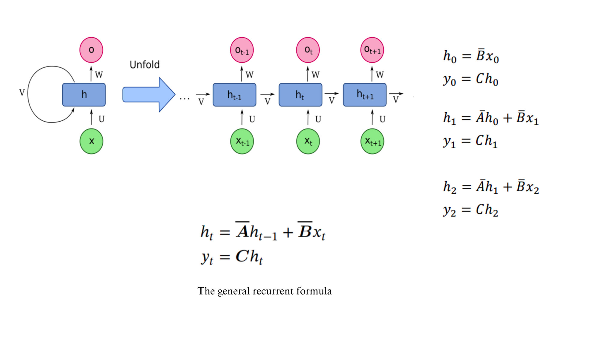
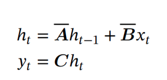
Recall how RNNs operate. Each RNN block expects a current input state and a previous hidden state to output the next hidden state and (optionally) an output state. So, do the equations in Figure 3, look like an RNN? Indeed, that is it. It takes the previous hidden state ht-1 and current input x_t to get the current hidden state h_t and output y_t.

Convolution

Now let’s try to understand the convolution aspect by doing some calculations.

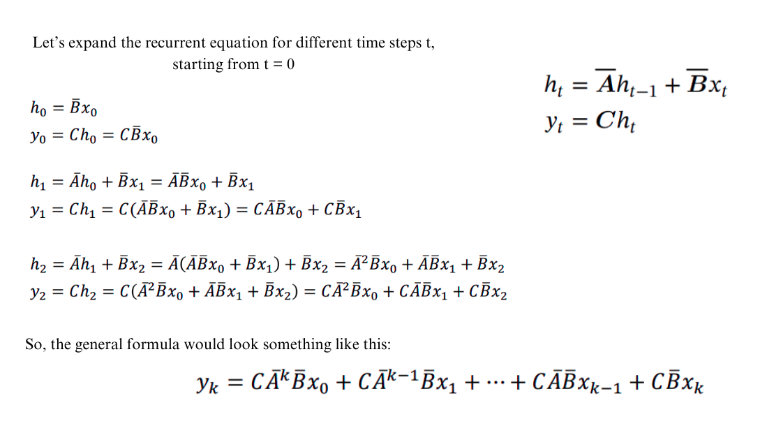
From the above figure, we can see that we got a pattern when expanding the recurrent equation. This general formula can be represented as continuous convolution with a fixed Kernel K, as shown in the figure below.

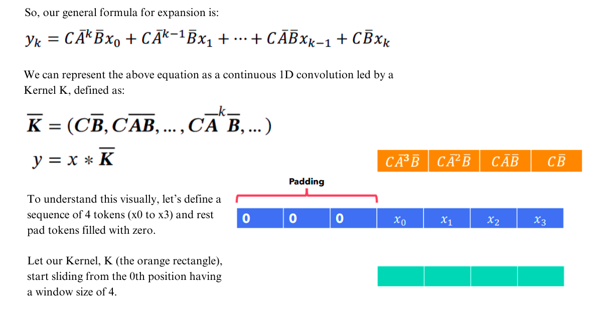
Now let’s see the visualization for the following set of tokens and we will recognize that we end up with the same equations as done in Figure 5-6.

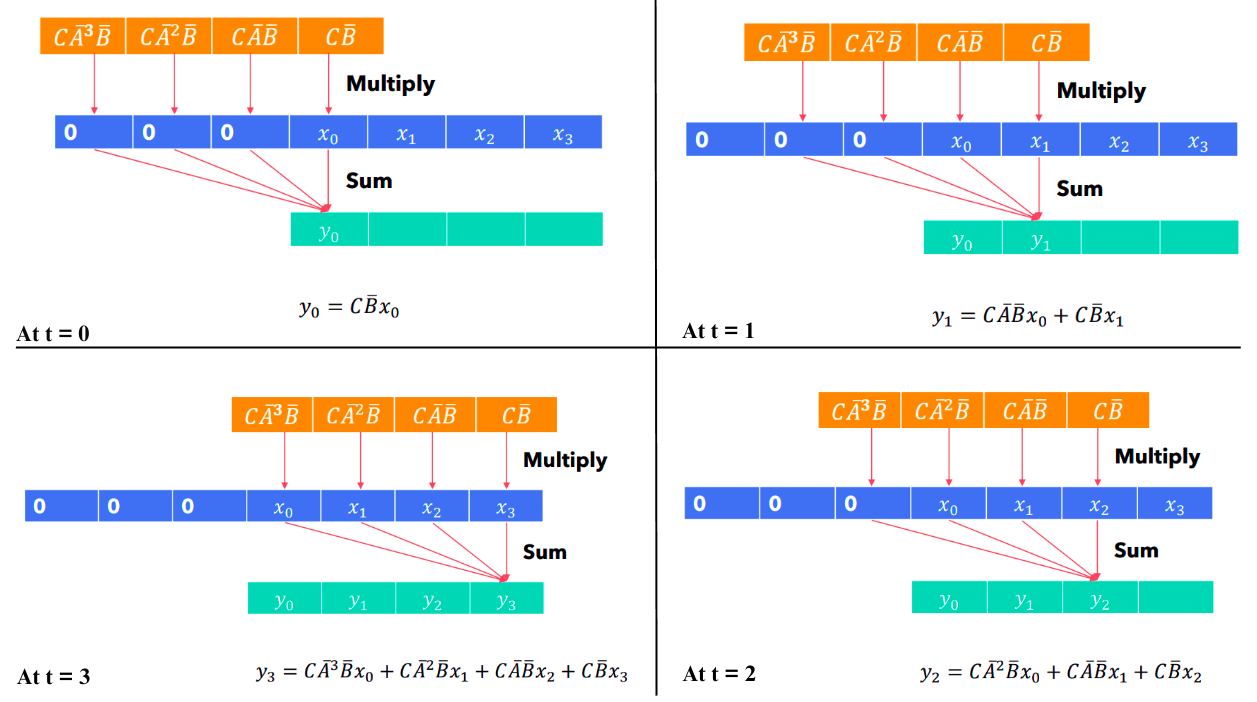
So, hopefully, at this point, we have a clear intuition and understanding of how we can represent the same representation with two different operations. The advantage of this is very simple, we can switch to convolution mode when we are doing training so that it can be parallelizable. During inference/decoding, we can switch to the recurrent mode for near-constant time inference. Please note here, that if you look at the kernels you can see that they are fixed. And since the kernels are fixed, so we can also term these models as “time-invariant” SSMs.

🦛 The HiPPO Matrix

Since SSM's behavior is very similar to Recurrent models, they performed poorly in practice, mostly because they also suffered from vanishing/exploding gradient descent problems. The prior work of S4 which was on Recurrent memory representation with optimal Polynomial Projections introduced us to the concept of HiPPO matrix. Remember the A matrix in Figure 1? We represent that A Matrix through HiPPO (in our case of S4 Model and Mamba). This (N x N) matrix allows us to memorize the history of inputs. This lower triangular matrix is defined like this:

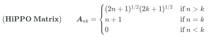
This above matrix helps to compress the history of the information. So, this A matrix in each hidden state memorizes its history. And the best part! It just needs to be computed once. Also, if you see, this is a lower triangular Matrix, this means it helps to mask out the next tokens (a replacement of Masked Self Attention). You might be having the question when I previously mentioned that the parameters are learnable. But the Matrix A seems to be precomputed, then where does the learning happen? The learnable matrix is A_bar. The last equation in Figure 2, shows that A_bar is associated with A and ∆. That ∆ is set to be learnable, but since that is attached to A and eventually with B, so A_bar and B_bar become learnable too.

The way the matrix A represents the latest memory history is mainly by keeping track of the coefficients of a Legendre polynomial. To understand more, please see the figure below.

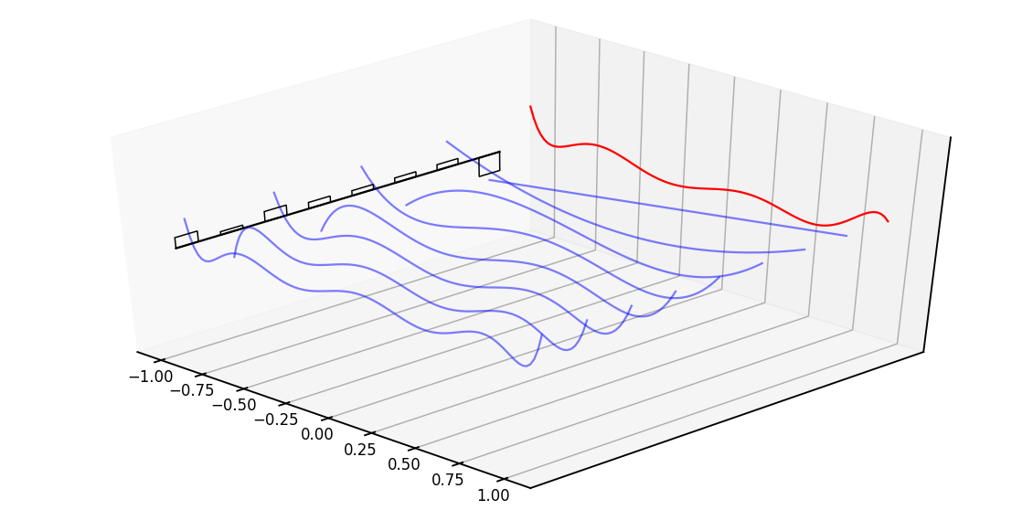
Right now, just forget language modeling for once. Consider this red signal as our target signal which we want to memorize or approximate. The black boxes represent the value of each state, and based on that state value, the blue line draws the Legendre series. With the passing of each step, the HiPPO matrix updates each step. The more recent the step, the better the approximation, and the lesser when the time step gets longer. In terms of language modeling, now think of each step as an addition of new tokens and tracking of its history.

🤔 What went wrong with S4?

The fundamental problem in sequence modeling is compressing the context into a smaller learnable state representation. And there lies a tradeoff between efficiency vs quality of state representation. For example, the transformer is inefficient (the fact that KV caches are required to explicitly store context) but is good with storing and representing long-form context. Whereas Recurrent models are efficient because they have finite states (~ constant time) they are less effective in context compression quality. S4 and all the other State Space Models are not very good at some tasks like Selective Copying and In-context Learning. So, in one word, they fail to do content/context-aware reasoning. The Mamba paper is on solving those two problems. Let’s discuss this in more detail.

🐍 Enter The Mamba

Vanilla SSMs or S4 models do not perform well on the following synthetic tasks:

1. Selective Copying: In the context of a language model, selective copying refers to the ability to discern relevant information from a given input and reproduce or incorporate it appropriately in the generated output. It involves the model's capability to identify and reproduce specific phrases, entities, or patterns from the input data, enhancing the relevance and coherence of the generated text.
2. Induction Heads: Induction heads in a language model pertain to specialized components that facilitate the model's capacity to infer and generalize knowledge from the input data. Similar to how humans draw conclusions and make inferences based on observed patterns, induction heads enable the model to extrapolate information, understand underlying relationships, and apply learned concepts to generate more nuanced and contextually appropriate responses.

Selection Mechanism

Let’s start with this example. Suppose you give a tweet (which is filled with some bad words) and you expect to get a filtered tweet (without changing the main tweet subject but rid of those words). Today’s transformer-based models can do those (by basically learning, the attention pattern of those words and the instruction to follow context-aware completion) but current SSM models fail to do so. Basically, in this task, all you need to be to copy-paste the take but selectively.

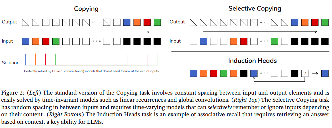
Look at Figure 10 carefully and now you can understand the difference between both the tasks (left and right). The reason why vanilla SSMs fail to learn Selective Copying tasks is because they are time-invariant (Remember: Kernel is fixed). This means that the learnable parameters remain fixed with the incoming of each new token.

This is the first change that Mamba introduced in an operation called Selective Scan. Please note this is a point where it diverges from S4. This “Selective Scan” operation now, does not hold the dual property of convolution and recurrence. Hence, Mamba relies on recurrence only. Because of time-variant parameterization. The Matrix A (HiPPO matrix) remains the same, but ∆, B and C now become the functions of the input. The figure below shows the difference in the selection mechanism (or the working difference of S4 vs Mamba).

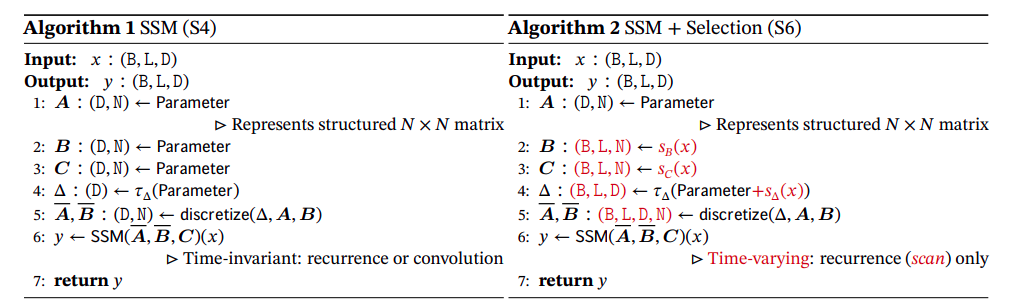
In the above figure, till A, everything remains the same. Where B is Batch size, L is the sequence/context length and D is the embedding dimension. Here, instead of treating B, and C as parameters like S4, they are the output of some projections. Here is an awesome implementation from the Mamba Minimal repository.

import torch 

def ssm(self, x):
    """Runs the SSM. See:
        - Algorithm 2 in Section 3.2 in the Mamba paper [1]
        - run_SSM(A, B, C, u) in The Annotated S4 [2]


    Args:
        x: shape (b, l, d_in)    (See Glossary at top for definitions of b, l, d_in, n...)

    Returns:
        output: shape (b, l, d_in)


    Official Implementation:
        mamba_inner_ref(), https://github.com/state-spaces/mamba/blob/main/mamba_ssm/ops/selective_scan_interface.py#L311
        
    """
    (d_in, n) = self.A_log.shape


    # Compute ∆ A B C D, the state space parameters.
    #     A, D are input independent (see Mamba paper [1] Section 3.5.2 "Interpretation of A" for why A isn't selective)
    #     ∆, B, C are input-dependent (this is a key difference between Mamba and the linear time invariant S4,
    #                                  and is why Mamba is called **selective** state spaces)
    
    A = -torch.exp(self.A_log.float())  # shape (d_in, n)
    D = self.D.float()


    x_dbl = self.x_proj(x)  # (b, l, dt_rank + 2*n)
    
    (delta, B, C) = x_dbl.split(split_size=[self.args.dt_rank, n, n], dim=-1)  # delta: (b, l, dt_rank). B, C: (b, l, n)
    delta = F.softplus(self.dt_proj(delta))  # (b, l, d_in)
    
    y = self.selective_scan(x, delta, A, B, C, D)  # This is similar to run_SSM(A, B, C, u) in The Annotated S4 [2]
    
    return y

🎯 The Parallel Scan Operation

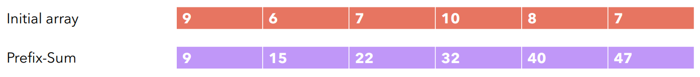
In Figure 11 (right), you can observe that, The Mamba paper coin the SSM operation as a scan operation. In this section what does this scan operation mean? Right now, you might have a proper understanding of why in Mamba only recurrent operation is used but not convolution. Since now the SSM operation is recurrent, it only holds the property of RNNs, for which training cannot be parallelizable. But still, the author of the Mamba paper finds some room for improvement. If you are familiar with basic Data Structures and Algorithms, then you might have heard about the problem called “The Prefix Sum” problem. It’s simple, you will be given an input array with some numbers. Each index of the output array should be a summation of all its previous indices. Here is an image to get some more details.

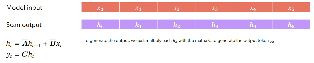
Does this operation look familiar? It’s similar to how RNN computes too. Each new state is the sum of the current input (xt) and previous state (ht-1) which is the recursive sum of all the previous states till now. Something like this:

This prefix-sum operation over arrays is also known as scan operation. So, a naive solution of this algorithm is simply to loop through the array and keep track of a prefix sum and each new sum will be prefix sum + current input. This gives us a time complexity of O(N) and so not parallelizable. That’s where the optimized version comes into place. The name of that algorithm is called Parallel Scan. Take a look at the figure below to understand how it works:

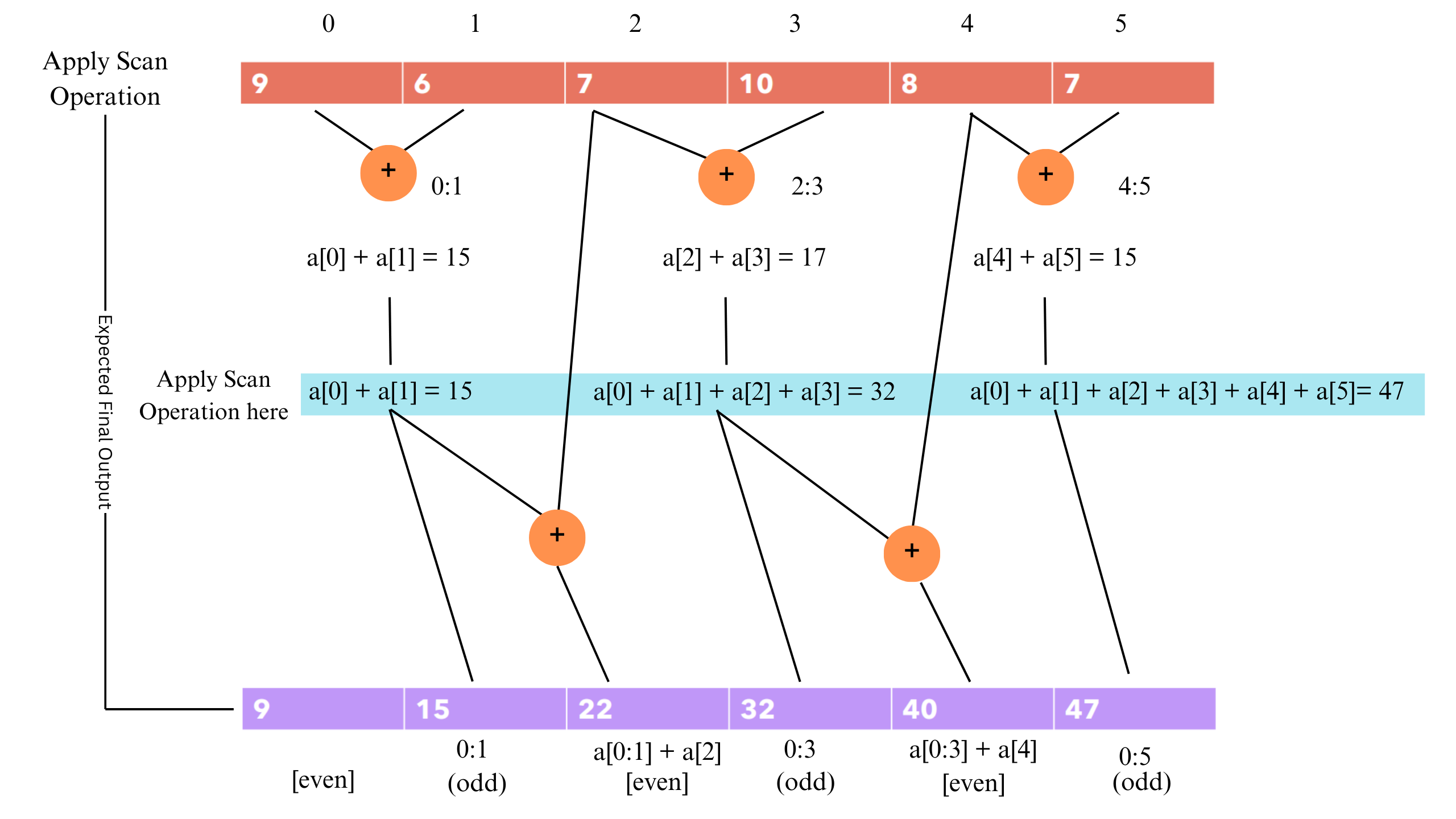
If you observe this, then you can find this algorithm simple to understand. For obvious reasons, the first value (0th index) should be given. Here are the three steps to compute this:

1. First, compute the intermediate corresponding sums. That is (0,1), (2,3), and so on…
2. Next, compute the prefix sum (or the scan operation) on these intermediate sums. To make things interesting you can recursively apply this function. But let’s not go into that depth. This gives us the prefix sum of all the odd indices.
3. Computing scans for even indices is simple. Just add the next term with the odd prefix sum. That is [(0,1) +2], [(3,4) + 5] and so on…

Interestingly, this way is only possible due to the associative property of the sum operations. Hence, we can spawn multiple threads (workers) to compute those intermediate steps and merge results. Hence our complexity reduces from O(N) to O(N/T) Where T is the number of threads.

🔍 Mamba: Selective Scan

Since Mamba is not parallelizable (Because it is time-variant), so we need to rely on recurrent operations. The Authors of Mamba had taken the optimization of recurrent operation speed up to a whole new level. Essentially by adopting three classic techniques.

1. Parallel Scan Algorithm
2. Kernel Fusion
3. Activation Recomputation.

We already discussed the parallel scan algorithm, which was the first level of optimization. In this section, we will discuss Kernel Fusion and the Activation Recomputation method, which makes the model more efficient.

Kernel Fusion

Before understanding Kernel Fusion, you should have a basic understanding of the GPU memory hierarchy and specifically should know terms like DRAM/HBM, SRAM, etc. If not, we have covered all of those in our previous blog. For Mamba, the scan operation is considered a memory-bound operation. So, Kernel Fusion is used to reduce the amount of memory IOs (i.e. loading from HBM to SRAM and vice versa). The SSM parameters A, ∆, B, and C are loaded from HBM to SRAM first, and then the discretization operation (i.e. conversion of A_bar and B_bar, from A, ∆, B, C) and recurrence operations are done in SRAM and then the final outputs are sent back to HBM.

Activation Recomputation

A Deep Learning model is nothing but a sequence or a series of matrix operations (like Multiplication, Addition, element-wise operations, etc). In any deep learning model training, there are two steps, Forward and Backward step. In the Forward step, we compute the intermediate values of each layer and the output and in the backward step or backpropagation, we compute the gradients of our parameters (w.r.t our loss) and update it. All of these operations can be represented as a computation graph.

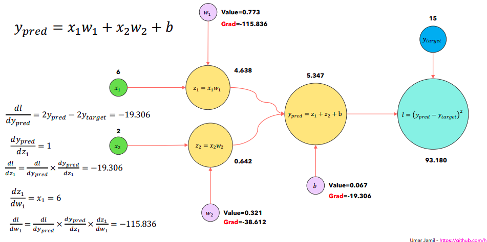
Through the use of this computation graph, we keep track of all the intermediate values and also can leverage novel algorithms like AutoGrad. However in the backward steps, since we require intermediate forward step values, a lot of memory is consumed during the process and gets more with more deeper neural network.

And, as you now know those intermediate values have to be loaded from HBM to SRAM before doing actual computation with it. And this takes more memory and time. So to reduce that, a simple optimization is done where all the intermediate values are not stored but are recomputed during the time of backward propagation when inputs are loaded from HBM to SRAM. This decreases the memory requirements by many folds.

🏛️ The Mamba Architecture

Till now we have discussed all the low-level optimization that the authors of the Mamba paper have used. So all the complicated parts end here. Now let’s take a brief overview of the Mamba model. We will first look into how one single Mamba block operates followed by the overall architecture.

The Mamba Block and Architecture

The Mamba model is made by stacking multiple layers of Mamba blocks, which is very similar to the stacked layer of the Transformer model. The architecture of the Mamba block is heavily inspired by the Hungry Hungry Hippo (H3) Architecture. Take a look at the figure below.

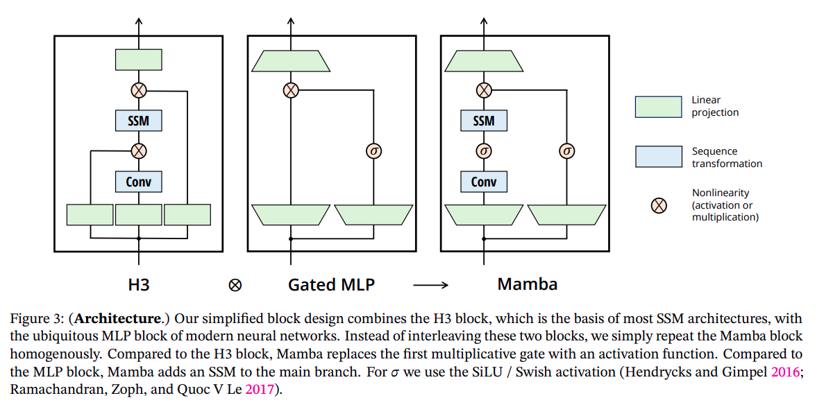
In the above figure, we can see that, the mamba block is the combination of H3 and Gated MLP Operations. It starts with projecting the inputs to a hidden state dimension, followed by convolution over the projected dimensions, with non-linearity (Which is the SILU activation function here). Then, we compute the SSM operation (discussed in previous sections). Followed by we then do a skip connection operation (Remember in the S4 section where we termed D as skip connection). Finally, we downscale our tensors with another linear projection and we are done. Here is the full architecture to understand more details.

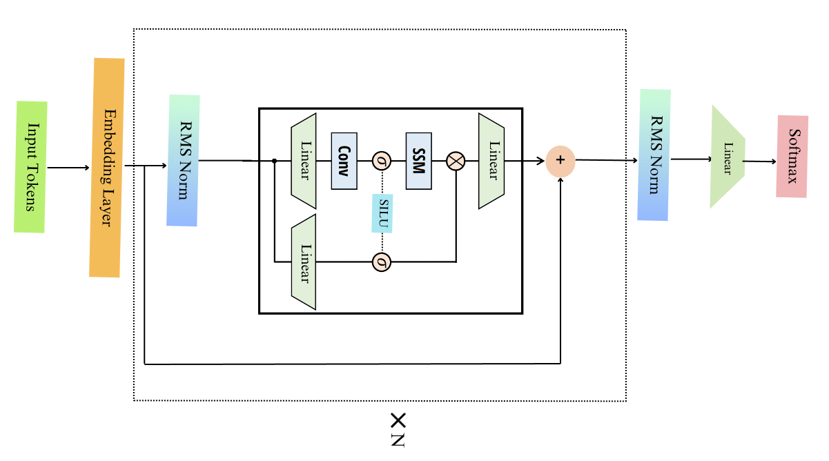
As you see in the above figure, it is very similar to the Transformer Architecture. We start with the normal input tokens. It uses the GPT-NeoX Tokenizers (Same as the Phythia Model). The tokens go inside an embedding layer, followed by the Mamba block, which starts from the RMS-Norm first then goes to the block explained above and this gets repeated (say N times), and finally, an RMS-norm, a projection, and then a Softmax to get the next token.

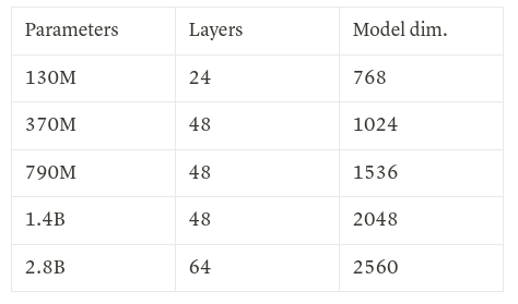
Training of Mamba

Mamba models come up with a lot of variants like mamba-130m, mamba-370m, mamba-790m, mamba-1.4b, mamba-2.8b. All of these models were trained on 300B tokens on the Pile dataset. An additional model mamba-2.8b-slimpj is trained on 600B tokens on the SlimPajama dataset. The model dimensions that were used are standard, as shown in the figure below.

📊 How does it compare with the current LLMs/SLMs

Out of all the 5 variants discussed above, we will see how these three variants viz, 130M, 790M, and 2.8B perform when compared with the present best 7B models like Llama 2, Mistral, etc. Here is the quick visualization for popular benchmarks like Piqa, Winogrande, Lambada, Hellaswag, Arc Challenge, etc.

The results are amazing given the size of the model and a model that works fundamentally differently than Transformer models. Here is another evaluation table of the paper comparing different models (similar to Mamba’s size) with different benchmarks.

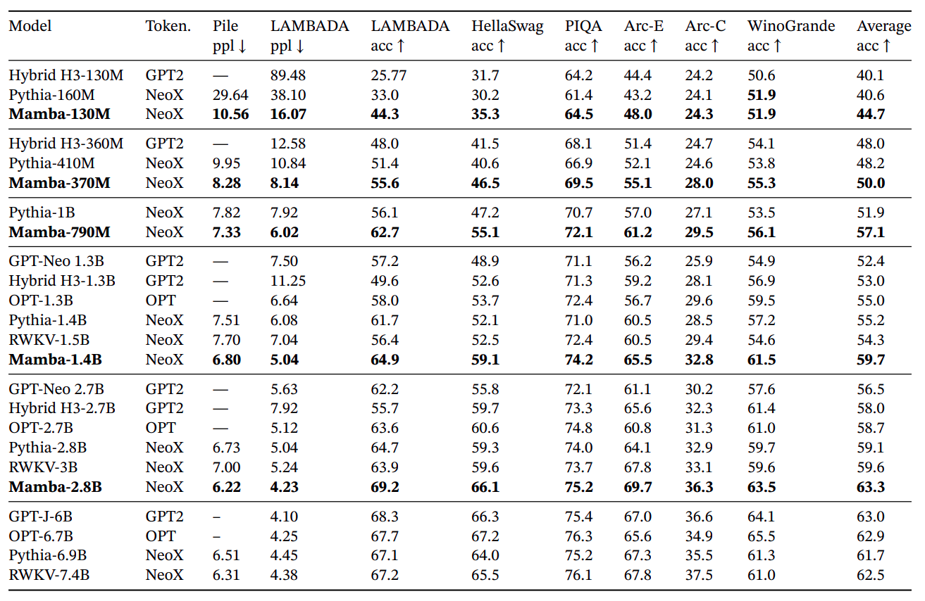
And as we can see from the above table we can see that Mamba outperforms all the other similar-sized models with ease. However, one thing to note that, it is still can not touch the numbers of Models like Mistral. However, the comparison is still incomplete before taking a look at the speed and memory benchmarks. The figure below shows the comparison of different implementations (Attention, Scan operations, etc) w.r.t Time (in ms) and Throughput (tokens/seconds).

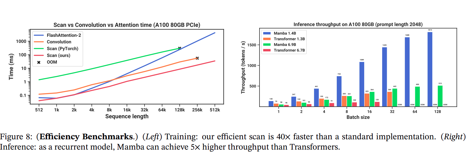
The above figure clearly shows us the advantage of performance speedup when Scan operation is used vs Flash Attention v2 (Which has become the current standard when Transformer-based LLMs are implemented). Overall shows a huge promise in terms of domain-based usages of the models with a very small number of parameters and greater speed.

🌀 Conclusion and Future Work of Mamba

The Mamba architecture (derived from S4) and a fresh Attention-free architecture gives us a huge lesson: for one problem (like Sequence Modelling), there could be multiple effective solutions. Sure, Mamba is a bit difficult to understand since its underlying concepts come from State Space Modelling and Control Engineering, but it sure shows very promising results in the very first iteration. Not only that, the paper shows that Mamba holds similar performances in any Sequence to Sequence tasks, other than language modeling, like DNA Modelling, Audio Generation, etc. Mamba can be a very strong candidate in the ongoing revolution of Small Language Models. In the next blog we will try to see and compare that with all other existing and popular Small Language Models like Phi1/1.5/2 Stable LM-2 etc. So stay tuned.

📜 References

• Mamba: Linear-Time Sequence Modeling with Selective State Spaces
• Structured State Space Models for In-Context Reinforcement Learning
• Umar Jamil's Video Slides on Mamba.
• The Annotated S4
• Transformer KV caching explained.
• Hungry Hungry Hippos: Towards Language Modeling with State Space Models
• Sigmoid-Weighted Linear Units for Neural Network Function Approximation in Reinforcement Learning
• Mamba vs 7B by ZenoML.
• FlashAttention-2: Faster Attention with Better Parallelism and Work Partitioning
• In-context Learning and Induction Heads
• Automatic Differentiation in Pytorch.